Parallel R with the future package
In R, numerous packages can be used to parallelize code (parallel, snow, foreach, etc.), but each of these packages use unique syntaxes and none of them work for all cases of parallelization. Instead, the future package solves this problem! Briefly (see the future package for details), the future package works in three steps:
- Choose how you want to parallelize your code
- set the type of parallelization with the
plan()object.
- set the type of parallelization with the
- Choose which part of the code you would like to run in parallel
- place the part of the code that will be iterated within the
future({})object.
- place the part of the code that will be iterated within the
- Evaluate the code.
- run the iterations using the
value()object.
- run the iterations using the
The power of the future package is it separates the planning for the parallelization (steps 1 and 2) and then executes the code afterwards. This allows the user to control how and where to parallelize their code. Thus, the framework can be extended to any iterative process.
Table of Contents
- Packages
- For-loop Example and basic structure
- Tidyverse example using the furrr package
- Bayesian example using multiple nodes via the future.batchtools package
- Appendix: Testing speed of Future
Packages
Before you run the code, I recommend installing R 4.5 and IRKernel via conda. Once you activate your conda environment, feel free to run the rest through jupyter: https://easley.alliance.unm.edu/jupyter or https://hopper.alliance.unm.edu/jupyter
Final note: make sure you are on a node with 8 cores on an interactive node or logged into Jupyter before running the code.
# Load miniconda
module load miniconda3/latest

# create r_parallel which installs 4
conda create -n r_parallel_tutorial r=4.5 r-irkernel -c conda-forge

# enables you do use conda activate
eval "$(conda shell.bash hook)"

conda activate r_parallel_tutorial
# double check you have multiple cores available

install.packages(
    c("future", "batchtools", "future.batchtools", "repurrrsive",
      "purrr","dplyr","furrr","tidyr", "snow", "ggplot2",
      "tibble", "labeling", "farver","backports"),
    repos='http://cran.us.r-project.org',
    Ncpus = 8 )
also installing the dependencies ‘colorspace’, ‘hms’, ‘prettyunits’, ‘munsell’, ‘RColorBrewer’, ‘viridisLite’, ‘globals’, ‘listenv’, ‘parallelly’, ‘base64url’, ‘brew’, ‘checkmate’, ‘data.table’, ‘fs’, ‘progress’, ‘R6’, ‘rappdirs’, ‘stringi’, ‘withr’, ‘magrittr’, ‘generics’, ‘tidyselect’, ‘cpp11’, ‘gtable’, ‘isoband’, ‘scales’, ‘pkgconfig’


Updating HTML index of packages in '.Library'

Making 'packages.html' ...
 done
library(future) # needed for all examples
library(purrr) # needed for tidyvese example
library(dplyr) # needed for tidyverse example
library(furrr) # needed for tidyverse example
library(repurrrsive) # loads in data for tidyverse example
library(future.batchtools) # needed for bayesian example
library(tidyr) # needed for tidyverse example
library(snow) # needed to load Hmsc for bayesian example
library(ggplot2) # needed to plot functions
library(labeling) # needed to plot functions
library(farver) # needed to plot functions


# double-check you have access to mulitple cores
availableCores()

# check that you can run multicore (will fail for R-studio and windows!)
supportsMulticore()
Attaching package: ‘dplyr’


The following objects are masked from ‘package:stats’:
The following objects are masked from ‘package:base’:
system: 8
TRUE
R version 4.1.0 (2021-05-18)
Platform: x86_64-conda-linux-gnu (64-bit)
Running under: CentOS Linux 7 (Core)

Matrix products: default
BLAS/LAPACK: /users/mimann/.conda/envs/r_parallel_tutorial/lib/libopenblasp-r0.3.17.so

locale:
 [1] LC_CTYPE=en_US.UTF-8       LC_NUMERIC=C
 [3] LC_TIME=en_US.UTF-8        LC_COLLATE=en_US.UTF-8
 [5] LC_MONETARY=en_US.UTF-8    LC_MESSAGES=en_US.UTF-8
 [7] LC_PAPER=en_US.UTF-8       LC_NAME=C
 [9] LC_ADDRESS=C               LC_TELEPHONE=C
[11] LC_MEASUREMENT=en_US.UTF-8 LC_IDENTIFICATION=C

attached base packages:
[1] stats     graphics  grDevices utils     datasets  methods   base

other attached packages:
 [1] farver_2.1.0             labeling_0.4.2           ggplot2_3.3.5
 [4] snow_0.4-3               tidyr_1.1.3              future.batchtools_0.10.0
 [7] repurrrsive_1.0.0        furrr_0.2.3              dplyr_1.0.7
[10] purrr_0.3.4              future_1.21.0

loaded via a namespace (and not attached):
 [1] pillar_1.6.2      compiler_4.1.0    prettyunits_1.1.1 progress_1.2.2
 [5] base64enc_0.1-3   tools_4.1.0       digest_0.6.27     uuid_0.1-4
 [9] gtable_0.3.0      jsonlite_1.7.2    evaluate_0.14     lifecycle_1.0.0
[13] tibble_3.1.3      checkmate_2.0.0   pkgconfig_2.0.3   rlang_0.4.11
[17] IRdisplay_1.0     IRkernel_1.2      parallel_4.1.0    withr_2.4.2
[21] repr_1.1.3        rappdirs_0.3.3    hms_1.1.0         generics_0.1.0
[25] vctrs_0.3.8       globals_0.14.0    grid_4.1.0        tidyselect_1.1.1
[29] data.table_1.14.0 glue_1.4.2        listenv_0.8.0     R6_2.5.0
[33] fansi_0.4.2       parallelly_1.27.0 base64url_1.4     pbdZMQ_0.3-5
[37] magrittr_2.0.1    scales_1.1.1      backports_1.2.1   codetools_0.2-18
[41] batchtools_0.9.15 ellipsis_0.3.2    htmltools_0.5.1.1 colorspace_2.0-2
[45] brew_1.0-6        utf8_1.2.2        stringi_1.7.3     munsell_0.5.0
[49] crayon_1.4.1
1. For-loop example and basic structure
This example shows how the future package can be used for running a for-loop that iterates over a very slow function.
Setting up and running loop in serial
First, we will create a function that pauses for 0.5 seconds. At the end, we will print the length of time it took to run.
# custom function that waits a half a second and then prints current step value
slow_function <- function(step){

  # wait half a second
  Sys.sleep(.5)
    paste0("Step ", step, " completed")

}


#### running loop in serial ####
# timestamp before loop
t1 <- proc.time()
# pre-allocate output
output <- rep(NA, 50)

# for-loop
for (i in 1:50){
  output[i] <- slow_function(i)

}

# print the output for first 6 steps
head(output)

# timestampe after loop
t2 <- proc.time()


print("Elapsed time (seconds) for for-loop")
# length of time
time_Elapsed <- t2[[3]] - t1[[3]]
round(time_Elapsed, 2)
- 'Step 1 completed'
- 'Step 2 completed'
- 'Step 3 completed'
- 'Step 4 completed'
- 'Step 5 completed'
- 'Step 6 completed'
[1] "Elapsed time (seconds) for for-loop"
25.06
Rerunning for-loop in parallel
Now we will re-write the for-loop so it is compatible with future. We will choose to run it across every core in the node we are using.
WARNING: if you plan to run this example locally on R-studio, you will need to change it to plan(multisession).
1. Choose how you want to parallelize your code
using the plan() object set to "multicore", we will establish we want to use all the cores available on the node.
We will set the number of iterations to run to 50 and pre-allocate space for the future loop by creating the "command_set" object. Since future puts every iteratation in a list, we will use a vector to pre-allocate empty lists for every iteration.
#### rerunning loop in parallel using all available cores ####
# going to send iterations to each cores
# to run it only on specified number of cores, add the argument, workers.
plan(multicore)

iterations <- 50
# rewrite loop so it works with future:
# future requires the iterative step to be saved as its own list,
# thus we will create a list object with 50 slots for each step.
command_set <- vector(mode = "list", length = iterations)
2. Choose which part of the code you would like to run in parallel
Here, we are rewriting the for-loop to work with future.
We will place the section we want to iterate within the curly-brackets of the future() object. The output is written to a separate list within the y object (it creates a list of lists). When you run this code, it doesn't evaluate the loop but sets up the environments for each iteration to run in parallel. Thus, the time elapsed is all the time needed to plan the code.
WARNING: Setting up the lists prior to evaluation can slow down the parallelization effort (see appendix).
t1 <- proc.time()
for (i in 1:iterations){

  command_set[[i]] <- future(
    # code for each iteration within the curly brackets
    {slow_function(i)}
  )
}


t2 <- proc.time()


print("Elapsed time (seconds) for planning command set")
# length of time
time_Elapsed <- t2[[3]] - t1[[3]]
round(time_Elapsed, 2)
[1] "Elapsed time (seconds) for planning command set"
11.27
Before Future evaluates the R code, it first writes the global environment to the "command_set" object. Each iteration is one list, thus extracting the first list will display what it will do for the first step in the loop.
[1] "What one iteration looks like in the command set"


MulticoreFuture:
Label: ‘<none>’
Expression:
{
bash
slow_function(i)
}
Lazy evaluation: FALSE
Asynchronous evaluation: TRUE
Local evaluation: TRUE
Environment: R_GlobalEnv
Capture standard output: TRUE
Capture condition classes: ‘condition’
Globals:
3. Evaluate the code
The value() object will take the list and run the code in parallel. Since the output is a list of lists, we can collapse it into an array with the unlist object.
# evaluate, distribute each iteration here
output <- value(command_set)

# ouput is here but separates lists.
print("list output")
head(output) # using head to limit output


# we can combine them into a vector using unlist()
print("array output")
head(unlist(output)) # using head to limit output
[1] "list output"
[1] "array output"
- 'Step 1 completed'
- 'Step 2 completed'
- 'Step 3 completed'
- 'Step 4 completed'
- 'Step 5 completed'
- 'Step 6 completed'
all in one block:
# plan
plan(multicore)

command_set <- vector(mode = "list", length = 50)
t1 <- proc.time()

for (i in 1:50){
  command_set[[i]] <- future(
    # but code for each iteration with curly brackets
    {slow_function(i)}
  )
}

# evaluate
output <- value(command_set)

# ouput is here
head(unlist(output))


# timestampe after loop
t2 <- proc.time()


print("Elapsed time for future example:")
# length of time
time_Elapsed <- t2[[3]] - t1[[3]]
round(time_Elapsed, 2)
- 'Step 1 completed'
- 'Step 2 completed'
- 'Step 3 completed'
- 'Step 4 completed'
- 'Step 5 completed'
- 'Step 6 completed'
[1] "Elapsed time for future example:"
11.85
2. Tidyverse example using the furrr package
To change tidyverse code, all that is needed is to set up the parallelization (plan object) and then replace the map object with future_map. The evaluation step is completed with the future_map object.
Setup
This example uses the gapminder dataset and creates a linear model for each country. The datafame becomes a nested dataframe by country so we can use the purrr package to iterate over each country and compute the linear model. See this link to the purrr package and the repurrrsive for more details.
# create a nested dataframe with each country as a row
# we will iterate using the map function from the purrr package
head(gap_simple)


country_nested <-
  gap_simple %>%
  group_by(country) %>%
  nest() %>%
  ungroup() # this is necessary or furrr will be slow


# linear model we will run for each country.
# in the real world, don't do this!! Always check model assumptions!
custom_model <-
  function(data){
    # just to slow it down so its more obvious it's in parallel
    Sys.sleep(.2)
    lm(lifeExp ~ pop + gdpPercap + year, data = data)
  }


# Sequential form (normal purrr)
t1 <- proc.time()
model_done <-
    country_nested %>%
    mutate(lm_obj = map(data, custom_model))

t2 <- proc.time()
print("Elapsed time for sequential purrr  example:")
# length of time
time_Elapsed <- t2[[3]] - t1[[3]]
round(time_Elapsed, 2)
[1] "Elapsed time for sequential purrr example:"
28.92
Rerunning tidyverse in parallel via the furrr package
To change the code to work with tidyverse, replace the map object with future_map.
# using furrr package

# use all cores available
plan(multicore)

# this time we do no not need to the evauluation step as it is included in the future_map function.
t1 <- proc.time()
model_done <-
    country_nested %>%
    mutate(lm_obj = future_map(data, custom_model)) # switched map to future_map!

# switch back to one core
plan(sequential)
t2 <- proc.time()

print("Elapsed time for furrr example:")
time_Elapsed <- t2[[3]] - t1[[3]]
round(time_Elapsed, 2)
[1] "Elapsed time for furrr example:"
4.17
Example: model output for Bosnia and Herzegovina (proof the future code provided output).
Bosnia and Herzegovina
<summary style=display:list-item;cursor:pointer>
    <strong>Levels</strong>:
</summary>
<style>
.list-inline {list-style: none; margin:0; padding: 0}
.list-inline>li {display: inline-block}
.list-inline>li:not(:last-child)::after {content: "\00b7"; padding: 0 .5ex}
</style>
<ol class=list-inline><li>'Afghanistan'</li><li>'Albania'</li><li>'Algeria'</li><li>'Angola'</li><li>'Argentina'</li><li>'Australia'</li><li>'Austria'</li><li>'Bahrain'</li><li>'Bangladesh'</li><li>'Belgium'</li><li>'Benin'</li><li>'Bolivia'</li><li>'Bosnia and Herzegovina'</li><li>'Botswana'</li><li>'Brazil'</li><li>'Bulgaria'</li><li>'Burkina Faso'</li><li>'Burundi'</li><li>'Cambodia'</li><li>'Cameroon'</li><li>'Canada'</li><li>'Central African Republic'</li><li>'Chad'</li><li>'Chile'</li><li>'China'</li><li>'Colombia'</li><li>'Comoros'</li><li>'Congo, Dem. Rep.'</li><li>'Congo, Rep.'</li><li>'Costa Rica'</li><li>'Cote d\'Ivoire'</li><li>'Croatia'</li><li>'Cuba'</li><li>'Czech Republic'</li><li>'Denmark'</li><li>'Djibouti'</li><li>'Dominican Republic'</li><li>'Ecuador'</li><li>'Egypt'</li><li>'El Salvador'</li><li>'Equatorial Guinea'</li><li>'Eritrea'</li><li>'Ethiopia'</li><li>'Finland'</li><li>'France'</li><li>'Gabon'</li><li>'Gambia'</li><li>'Germany'</li><li>'Ghana'</li><li>'Greece'</li><li>'Guatemala'</li><li>'Guinea'</li><li>'Guinea-Bissau'</li><li>'Haiti'</li><li>'Honduras'</li><li>'Hong Kong, China'</li><li>'Hungary'</li><li>'Iceland'</li><li>'India'</li><li>'Indonesia'</li><li>'Iran'</li><li>'Iraq'</li><li>'Ireland'</li><li>'Israel'</li><li>'Italy'</li><li>'Jamaica'</li><li>'Japan'</li><li>'Jordan'</li><li>'Kenya'</li><li>'Korea, Dem. Rep.'</li><li>'Korea, Rep.'</li><li>'Kuwait'</li><li>'Lebanon'</li><li>'Lesotho'</li><li>'Liberia'</li><li>'Libya'</li><li>'Madagascar'</li><li>'Malawi'</li><li>'Malaysia'</li><li>'Mali'</li><li>'Mauritania'</li><li>'Mauritius'</li><li>'Mexico'</li><li>'Mongolia'</li><li>'Montenegro'</li><li>'Morocco'</li><li>'Mozambique'</li><li>'Myanmar'</li><li>'Namibia'</li><li>'Nepal'</li><li>'Netherlands'</li><li>'New Zealand'</li><li>'Nicaragua'</li><li>'Niger'</li><li>'Nigeria'</li><li>'Norway'</li><li>'Oman'</li><li>'Pakistan'</li><li>'Panama'</li><li>'Paraguay'</li><li>'Peru'</li><li>'Philippines'</li><li>'Poland'</li><li>'Portugal'</li><li>'Puerto Rico'</li><li>'Reunion'</li><li>'Romania'</li><li>'Rwanda'</li><li>'Sao Tome and Principe'</li><li>'Saudi Arabia'</li><li>'Senegal'</li><li>'Serbia'</li><li>'Sierra Leone'</li><li>'Singapore'</li><li>'Slovak Republic'</li><li>'Slovenia'</li><li>'Somalia'</li><li>'South Africa'</li><li>'Spain'</li><li>'Sri Lanka'</li><li>'Sudan'</li><li>'Swaziland'</li><li>'Sweden'</li><li>'Switzerland'</li><li>'Syria'</li><li>'Taiwan'</li><li>'Tanzania'</li><li>'Thailand'</li><li>'Togo'</li><li>'Trinidad and Tobago'</li><li>'Tunisia'</li><li>'Turkey'</li><li>'Uganda'</li><li>'United Kingdom'</li><li>'United States'</li><li>'Uruguay'</li><li>'Venezuela'</li><li>'Vietnam'</li><li>'West Bank and Gaza'</li><li>'Yemen, Rep.'</li><li>'Zambia'</li><li>'Zimbabwe'</li></ol>
Call:
lm(formula = lifeExp ~ pop + gdpPercap + year, data = data)

Coefficients:
(Intercept)          pop    gdpPercap         year
 -4.950e+02    4.916e-06   -5.017e-04    2.757e-01
3. Bayesian example using multiple nodes via the future.batchtools package
This example runs multiple Bayesian models in parallel by submitting each model (iteration) to a separate node. This is very useful because each model can already run in parallel, thus CARC enables you to run all of your Bayesian parallelized models at once. the future.batchtools packages will use information in the batchtools.torque.tmpl file in your current directory to submit jobs. This file can be modified to change parameters such as length of walltime, number of cores, etc (see file below).
These Bayesian models are joint-species distribution models (jSDMs) which fit the distributions of bird species and determines how it relates to their habitat, phylogeny, and traits. The code will run four Bayesian models that differ in their thinning and then write the models to file. The data and model objects are pre-built and loaded with the hmsc_setup.RData file and are derived from the bird example from their book.
For the sequential version, I already set up it using future. You can check your future code by running it sequentially by using plan(sequential).
batchtools.slurm.tmpl
batchtools.slurm.tmpl file needed in the same directory or specify the path to it. You will need this file created prior to running this example - see the future.batchtools Slurm template docs for the current format.
Setup
# bring in data for model
install.packages("coda")
install.packages("devtools") # if not yet installed
library(devtools)
install_github("hmsc-r/HMSC")
library(coda)
library(Hmsc)
load("hmsc_setup.RData")

# Setting up the model
studyDesign = data.frame(Route = XData$Route)
rL = Hmsc::HmscRandomLevel(sData=xy)
XFormula = ~ hab + poly(clim,degree = 2,raw = TRUE)
TrFormula = ~Migration + LogMass

# parameters for bayesian models.
nChains = 4
nParallel = 4
samples = 10
Updating HTML index of packages in '.Library'
Making 'packages.html' ...
done
also installing the dependencies ‘askpass’, ‘credentials’, ‘sys’, ‘zip’, ‘gitcreds’, ‘ini’, ‘fastmap’, ‘highr’, ‘markdown’, ‘xfun’, ‘diffobj’, ‘rematch2’, ‘clipr’, ‘curl’, ‘gert’, ‘gh’, ‘rprojroot’, ‘whisker’, ‘yaml’, ‘processx’, ‘mime’, ‘openssl’, ‘cachem’, ‘xopen’, ‘commonmark’, ‘knitr’, ‘Rcpp’, ‘stringr’, ‘xml2’, ‘brio’, ‘praise’, ‘ps’, ‘waldo’, ‘usethis’, ‘callr’, ‘desc’, ‘httr’, ‘memoise’, ‘pkgbuild’, ‘pkgload’, ‘rcmdcheck’, ‘remotes’, ‘roxygen2’, ‘rstudioapi’, ‘rversions’, ‘sessioninfo’, ‘testthat’
Updating HTML index of packages in '.Library'
Making 'packages.html' ...
done
Loading required package: usethis
Downloading GitHub repo hmsc-r/HMSC@HEAD
RcppArmad... (NA -> 0.10.6.0.0) [CRAN]
matrixStats (NA -> 0.60.0 ) [CRAN]
conquer (NA -> 1.0.2 ) [CRAN]
MatrixModels (NA -> 0.5-0 ) [CRAN]
SparseM (NA -> 1.81 ) [CRAN]
fansi (0.4.2 -> 0.5.0 ) [CRAN]
gridExtra (NA -> 2.3 ) [CRAN]
dotCall64 (NA -> 1.0-1 ) [CRAN]
plyr (NA -> 1.8.6 ) [CRAN]
quantreg (NA -> 5.86 ) [CRAN]
mcmc (NA -> 0.9-7 ) [CRAN]
maps (NA -> 3.3.0 ) [CRAN]
viridis (NA -> 0.6.1 ) [CRAN]
spam (NA -> 2.7-0 ) [CRAN]
truncnorm (NA -> 1.0-8 ) [CRAN]
statmod (NA -> 1.4.36 ) [CRAN]
sp (NA -> 1.4-5 ) [CRAN]
pROC (NA -> 1.17.0.1 ) [CRAN]
pracma (NA -> 2.3.3 ) [CRAN]
MCMCpack (NA -> 1.5-0 ) [CRAN]
FNN (NA -> 1.1.3 ) [CRAN]
fields (NA -> 12.5 ) [CRAN]
BayesLogit (NA -> 2.1 ) [CRAN]
ape (NA -> 5.5 ) [CRAN]
abind (NA -> 1.4-5 ) [CRAN]
Installing 25 packages: RcppArmadillo, matrixStats, conquer, MatrixModels, SparseM, fansi, gridExtra, dotCall64, plyr, quantreg, mcmc, maps, viridis, spam, truncnorm, statmod, sp, pROC, pracma, MCMCpack, FNN, fields, BayesLogit, ape, abind
Updating HTML index of packages in '.Library'
Making 'packages.html' ...
done
[32m✔[39m [90mchecking for file ‘/tmp/Rtmp7wOOGo/remotes4e4e7a4c3c6e/hmsc-r-HMSC-940f41c/DESCRIPTION’[39m[36m[36m (389ms)[36m[39m
[90m─[39m[90m [39m[90mpreparing ‘Hmsc’:[39m[36m[39m
[32m✔[39m [90mchecking DESCRIPTION meta-information[39m[36m[39m
[90m─[39m[90m [39m[90minstalling the package to process help pages[39m[36m[39m
[90m─[39m[90m [39m[90msaving partial Rd database[39m[36m[36m (19.7s)[36m[39m
[90m─[39m[90m [39m[90mchecking for LF line-endings in source and make files and shell scripts[39m[36m[39m
[90m─[39m[90m [39m[90mchecking for empty or unneeded directories[39m[36m[39m
[90m─[39m[90m [39m[90mbuilding ‘Hmsc_3.0-12.tar.gz’[39m[36m[39m
#!/bin/bash

## Job name:
#SBATCH --partition general
#SBATCH --nodes 1
#SBATCH --ntasks-per-node 4
#SBATCH --time 0:20:00
#SBATCH --job-name x_big_model_test_parallel_4_cores_4_chains
#SBATCH --output x_big_model_test.out
#SBATCH --error x_big_model_test.err
#SBATCH --mail-type end,fail


start=`date +%s`

cd $SLURM_SUBMIT_DIR

# load R
module load libdeflate/1.14-2pby r/4.5.2-pspo
export LD_LIBRARY_PATH=$LIBDEFLATE_LIB:$LD_LIBRARY_PATH

# if the driver session (e.g. a conda-based R kernel in JupyterHub) exported
# R_LIBS_USER, it points at that R's own personal library path (a different
# platform triplet than the module R), which shadows the module R's own
# default personal library and makes it unable to find batchtools. Unset it
# so the worker uses the module R's own default:
unset R_LIBS_USER

#Rscript -e '.libPaths("~/R/Jupyter")' -e 'batchtools::doJobCollection("<%= uri %>")'
Rscript -e 'batchtools::doJobCollection("<%= uri %>")'
end=`date +%s`

runtime=$((end-start))

echo "Runtime was $runtime seconds"
# this example runs sequentially (no scheduler submission) as a baseline
plan(sequential)

m = Hmsc(Y=Y, XData = XData, XFormula=XFormula,
         phyloTree = phyloTree, TrData = TrData,
         TrFormula = TrFormula,
         distr="probit", studyDesign=studyDesign,
         ranLevels=list(Route=rL))
y <- list()
t1 <- proc.time()
# running 4 models, each with a different thinning value
for (thin in c(2,3,4,5)){
  y[[thin]] <- future({
  transient = 50*thin
  m = sampleMcmc(m, thin = thin, samples = samples, transient = transient,
                 nChains = nChains, initPar = "fixed effects",
                 nParallel = nParallel)

  # write model outputs to file
  filename=file.path(paste0("Big_model_torque_chains_",as.character(nChains),"_samples_",as.character(samples),"_thin_",as.character(thin)))
  save(m,file=filename)
  }, seed = TRUE)
}
# evaluate expression
#y <- value(y)

t2 <- proc.time()
time_Elapsed <- t2[[3]] - t1[[3]]
round(time_Elapsed, 2)
875.1
Rerunning bayesian models in parallel using future.batchtools package
# set up that it will submit slurm scripts for each model
# calls upon the batchtools.slurm.tmpl file to set the parameters for each job

plan(batchtools_slurm)

m = Hmsc(Y=Y, XData = XData, XFormula=XFormula,
         phyloTree = phyloTree, TrData = TrData,
         TrFormula = TrFormula,
         distr="probit", studyDesign=studyDesign,
         ranLevels=list(Route=rL))

y <- list()
t1 <- proc.time()
# running 4 models, each with a different thinning value
for (thin in c(2,3,4,5)){
  y[[thin]] <- future({
  transient = 50*thin
  m = sampleMcmc(m, thin = thin, samples = samples, transient = transient,
                 nChains = nChains, initPar = "fixed effects",
                 nParallel = nParallel)

  # write model outputs to file
  filename=file.path(paste0("Big_model_torque_chains_",as.character(nChains),"_samples_",as.character(samples),"_thin_",as.character(thin)))
  save(m,file=filename)
  }, seed = TRUE)
}
# evaluate expression
y <- value(y)

t2 <- proc.time()
time_Elapsed <- t2[[3]] - t1[[3]]
round(time_Elapsed, 2)
setting updater$Gamma2=FALSE due to specified phylogeny matrix

setting updater$Gamma2=FALSE due to specified phylogeny matrix

setting updater$Gamma2=FALSE due to specified phylogeny matrix

setting updater$Gamma2=FALSE due to specified phylogeny matrix
375.03
Appendix: Testing speedup with Future
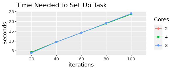
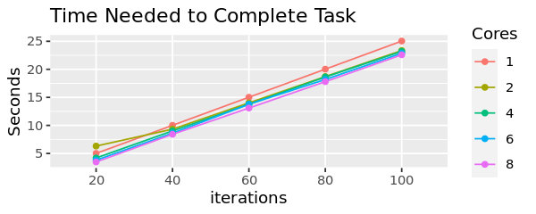
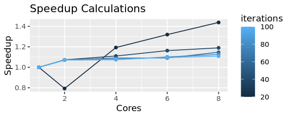
For some circumstances, writing your code in parallel with future package can make it slower! To illustrate this problem, I created a function called speedup_calc that allows you to play with the parameters and see what scenarios running the code in parallel. Essentially, it runs a for loop for different combinations of iterations, cores, and length of iterations (wait_time). Also, you can see the cost of setting up the code with the "evaluate" argument. When it is done, it will generate two plots (unless evaluate == FALSE), a plot showing how long it took for each iteration and core combination to complete, and a plot showing the speedup when the number of cores is increased.
Arguments:
* iterations requires a value (total iteratations) or a vector.
* cores requires numeric a vector of cores you want to run.
* wait_time requires a numeric value for how to wait for each iterative step.
* evaluate requires a TRUE or FALSE. Allows you to turn off evaluation if you only want to measure setup time. It will also skip the speedup plot since setup time cannot be calculated for the serial version.
speedup_calc function:
speedup_calc <-
    function(iterations, cores, wait_time, evaluate){

    try(if(cores[1] != 1) stop("Need to run the core as 1"))

    # set up arrays for storing for-loop data
        times <- array(dim = c(length(iterations), length(cores)))
        row.names(times) <- iterations


    # running the first set outside of the future loop.
    # skips it if since there is no set up time for serial version.
    if (evaluate == TRUE){

        j <- 1
        for (i in 1:length(iterations)){

            current_step <- iterations[i]
                    ### time point 1
            t1 <- proc.time()
            setup <- vector(mode = "list", length = length(iterations))

                 for (k in 1:current_step){

                        Sys.sleep(wait_time)
                    }


            ### time point
            t2 <- proc.time()

            ## calculate difference in time and convert to minutes. Write to array
            times[i, j] <- (t2[[3]] - t1[[3]])

                }


    }

        # loop that first run through the number of cores
        for (j in 2:length(cores)){

            plan(multicore, workers = cores[j])
            # figure out time it taakes for each iteration for j number of cores
            for (i in 1:length(iterations)){

                current_step <- iterations[i]
                ### time point 1
                t1 <- proc.time()
                setup <- vector(mode = "list", length = length(iterations))

                    for (k in 1:current_step){

                        setup[[k]] <- future({Sys.sleep(wait_time)})
                    }

                #  Allows you to run it without evaluating the code
                if (evaluate == TRUE){evaluated <-  value(setup)}

                ### time point
                t2 <- proc.time()

                ## calculate difference in time and convert to minutes. Write to array
                times[i, j] <- (t2[[3]] - t1[[3]])
            }


        }


        ### clean and plot all of the data
        options(repr.plot.width = 5, repr.plot.height = 2)
        # loop is finished so now cleanaing up data
        times <- as.data.frame(times)
        colnames(times) <- cores
        times$iterations <- row.names(times)

        times$iterations <- factor(as.character(iterations), levels = iterations)
        # plot time it takes for each core/iteratiaons combo

    if (evaluate == FALSE){
        time_plot <-
            times %>%
            pivot_longer(cols = 1:length(cores), names_to = "Cores", values_to = "Seconds") %>%
            filter(Cores != "1") %>%
            ggplot(aes(x = iterations, y = Seconds, group =  Cores, color = Cores)) +
            geom_line() + geom_point() +
            ggtitle("Time Needed to Set Up Task")
        print(time_plot)
        }


    if (evaluate == TRUE){

         time_plot <-
            times %>%
            pivot_longer(cols = 1:length(cores), names_to = "Cores", values_to = "Seconds") %>%
            ggplot(aes(x = iterations, y = Seconds, group =  Cores, color = Cores)) +
            geom_line() + geom_point() +
            ggtitle("Time Needed to Complete Task")
        print(time_plot)

        # speedup calcs
        speedup_df <- 1/ (times[,1:length(cores)] /times[,1] )
        speedup_df$iterations <- iterations


        speedup_plot <-
            speedup_df %>%
            pivot_longer(cols = 1:length(cores), names_to = "Cores", values_to = "Speedup") %>%
            mutate(Cores = as.numeric(Cores)) %>%
            ggplot(aes(x = Cores, y = Speedup, group =  iterations, color = iterations)) +
            geom_line() + geom_point() +
            ggtitle("Speedup Calculations")

        print(speedup_plot)
        }

    }
Scenario 1: Cost of setup for many iterations
This scenario plots how much time the setup takes. The cost for 100 iterations or more can be timely. The line with one core is omitted becauase it doesn't have setup time.
speedup_calc(iterations = seq(from = 20, 100, by = 20), cores = c(1,2, 4, 8), wait_time = .25, evaluate = FALSE)
Scenario 2: running previous example
Given the cost due to the setup time, parallelization offer very little improvement.
speedup_calc(iterations = seq(from = 20, 100, by = 20), cores = c(1,2, 4, 6, 8), wait_time = .25, evaluate = TRUE)
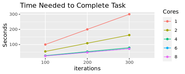
Scenario 3: Moderate speedup with a slower iteration
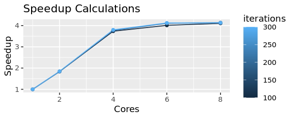
When you incease the wait_time to 1 second, the increase in cores does provide a benefit.
speedup_calc(iterations = seq(from = 100, 300, by = 100), cores = c(1,2,4,6, 8), wait_time = 1, evaluate = TRUE)
Scenario 4: Best scenario for speedup
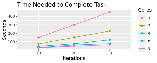
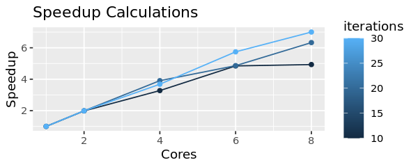
The best case for future will be running the code with few iterations but very slow functions.
speedup_calc(iterations = seq(from = 10, 30, by = 10), cores = c(1,2,4,6, 8), wait_time = 15, evaluate = TRUE)
Conclusion
The future package will offer the best performance when there are fewer iterations but each iteration is very slow. With your code, try running one iteration to see how long it takes and then use that estimate with speedup_calc. Depending on the wait_time and number of iterations, the function will give an estimate on if parallelization is worthwhile (caveat: the code will be slower if you have a large global environment).
Video walkthrough
Parallel R with Future — from the CARC video tutorials:
Migrated from UNM-CARC QuickBytes (last source update 2026-08-03). Spotted a problem? Open an issue or pull request.
Machine-readable versions of this page: Markdown twin · raw source on GitHub · llms.txt · llms-full.txt (whole site). See For AI agents.